Free Analog Filter Program
This Analog Filter Program can be used to design a low or high pass active filter from 2 to 12 poles and zeros and display the sinusoidal and transient characteristics of the filter.
The following filters are supported:
Butterworth
Bessel
Gaussian
Critically Damped
Legendre
Papoulis-Legendre
Chebyshev
Maximally Flat At Origin (Inverse Chebyshev)
Maximally Flat Beyond Origin
Elliptic (Cauer)
Transitional Butterworth-Bessel
Transitional Butterworth-Gaussian
Transitional Butterworth-Critically Damped
All filters are normalized for a cutoff frequency of 1 Hz.
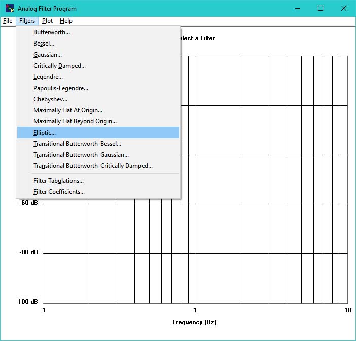
Select a Filter
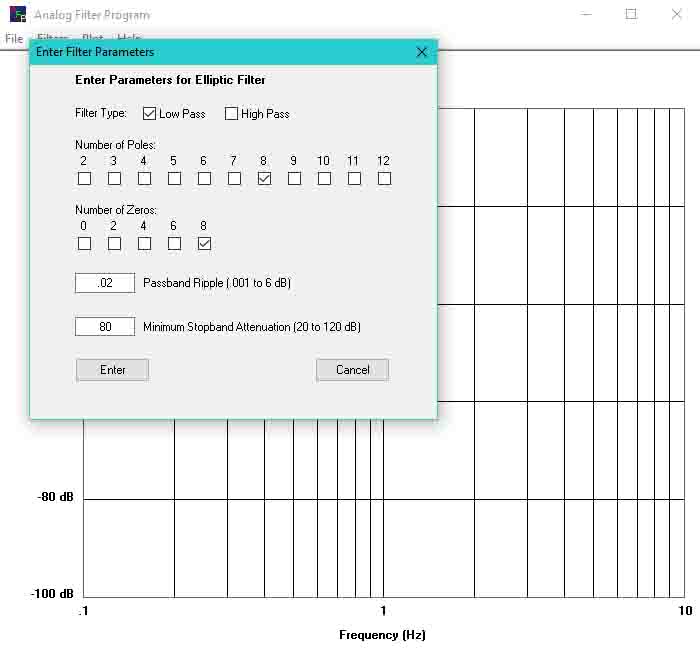
Enter Filter Parameters then click on Enter
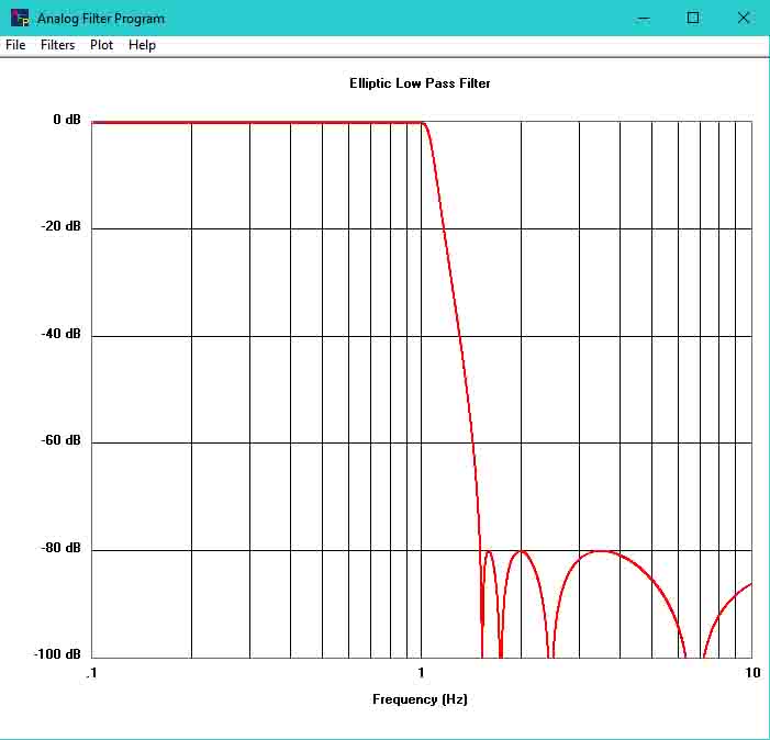
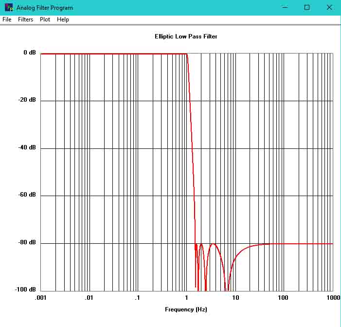
Display Filter Magnitude
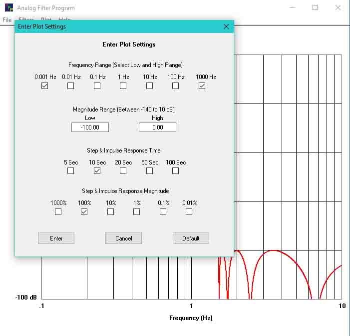
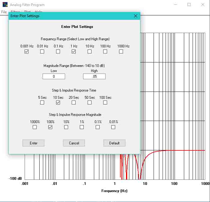
Change Frequency Range Plot Settings then click on Enter
Display New Plot Settings
Change Plot Settings to Display Passband Magnitude then click on Enter
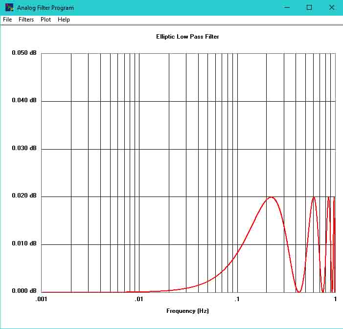
Display Passband Magnitude
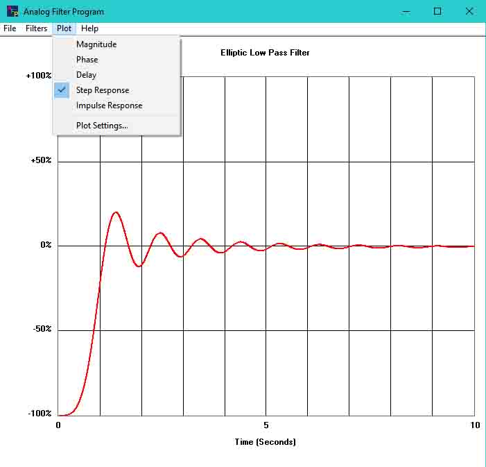
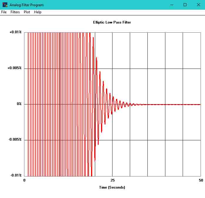
Display Step Response
Change Plot Settings to display Step Response Settling Time to less than 0.01% then click on Enter
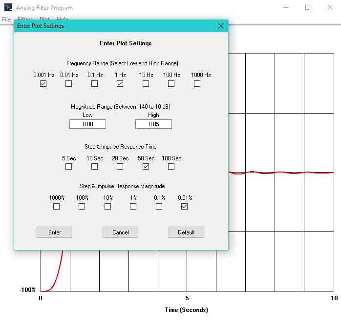
Display Step Response settling time to less than 0.01%
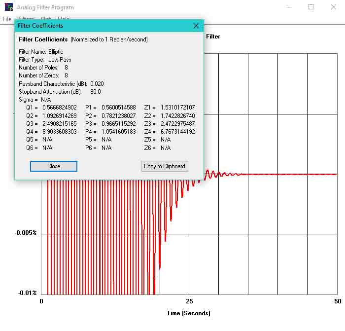
Display Filter Coefficients
In addition to the preceding examples the phase shift, delay and impulse responses can be displayed. The current graph display can be printed. A listing of the frequencies, magnitude, phase and delay in .01 Hz increments can be displayed and printed. Odometers are displayed on the lower left side of the window which shows the vertical and horizontal coordinates relative to the filter characteristic plot. Two or more copies of this program can be run at the same time to compare filters or display different characteristics of the same filter.
Program Operation:
Click on ‘Filters’ and then click on a filter name. This will bring up a window to enter the parameters for the filter name selected. After the parameters are entered click on ‘Enter’ and the filter characteristic will be displayed on the graph.
Odometers are displayed on the lower left side of the window which shows the vertical and horizontal coordinates relative to the filter characteristic plot if the cursor is on the graph and the window has focus.
To display a listing of the frequencies, magnitude, phase and delay in .01 Hz increments click on ‘Filters’ and then click on ‘Filter Tabulations’. The Filter Tabulations can be printed by clicking on ‘File’ and then ‘Print’ in the Filter Tabulations window.
To display the filter coefficients click on ‘Filters’ and then click on 'Filter Coefficients’. This will bring up a window that displays the filter parameters entered and the filter coefficients. Clicking on ‘Copy to Clipboard’ will copy the contents of the window to the clipboard where it can be pasted into Notepad or any word processing program etc.
To select the characteristic to be displayed on the graph, click on ‘Plot’ and then click on ‘Magnitude’, ‘Phase’, ‘Delay’, ‘Step Response’ or ‘Impulse Response’.
To change the plot settings click on ‘Plot’ and then click on ‘Plot Settings’. This will bring up the plot settings window. Clicking on ‘Default’ will reset the plot settings to their default values.
The current graph display can be printed by clicking on ‘File’ and then ‘Print’.
All the filters are normalized for a cutoff frequency of 1 Hz. To scale the filter for a frequency other than 1 Hz, multiply by the new frequency or divide the time by the new frequency. If the 1 Hz cutoff filter has a 2 second delay then an equivalent 1 KHz cutoff filter will have a (2 second/1 KHz) 2 milliseconds delay.
Plots:
Magnitude: Displays the magnitude plot of the filter in decibels versus frequency. The decibel is defined as 20 times the logarithm to the base ten of the ratio of the output magnitude divided by the input magnitude.
Phase: Displays the phase shift in degrees versus frequency. If the cursor is placed on the graph the odometers display the total phase shift versus frequency for the cursor position relative to the graph.
Delay: Displays the delay in seconds versus frequency. Delay is the rate of change of the phase shift. It is the first derivative of the phase shift with respect to the angular frequency.
Step Response: Displays the unit step function response in percent of the final value versus time.
Impulse Response: Displays the unit impulse response in percent of the final value versus time.
Notes:
Not all possible filter configurations are realizable. If the specified configuration is not realizable an error message will be displayed and the parameters can be modified for a new try. Some of the realizable filters may not be practical due to the high quality factor(s) required. These filters will have attenuation rates much greater than 6 dB per octave per pole and usually have high ripple or passband attenuation. Quality factors over 10 are usually not practical. This is a very arbitrary number and is dependent on the ratio of the cutoff frequency to the bandwidth of the amplifiers used in implementing the active filter and accuracy requirements.
The theoretical DC gain of low pass even-order unity gain filters that have ripple in the passband (Chebyshev, Maximally Flat Filters Beyond the Origin and Elliptic) will not be unity at DC but will be low by the amount of the ripple in the passband. The gain will be unity in the passband at the frequencies where the ripple is a maximum. This is usually not acceptable in practical applications as in most cases the DC gain is expected to be unity. Therefore, in most practical applications the filter is designed such that the gain is unity at DC and the ripple increases the gain by the amount of the ripple specification. When this is the case the cutoff frequency is defined as that frequency at which the last ripple prior to the start of the attenuation slope is zero decibels or unity gain. All low pass filters designed with this program have unity gain at DC.
Filter Types:
The first set of filters, Butterworth, Bessel, Gaussian, Legendre, Papoulis-Legendre and Chebyshev are polynomial filters. That is, there is an actual equation for each of these filters. These filters optimize one property such as delay or attenuation rate while degrading other properties such as the sinusoidal or transient responses. The next set of filters, Maximally Flat and Elliptic are a ratio of polynomials and are empirically designed (designed by trial and error).
Butterworth Low Pass Filter:
Considered to have good sinusoidal amplitude response in the passband and poor transient response characteristics. Characterized as being maximally flat at the origin (DC) and the attenuation at the cutoff frequency being one over the square root of two which is -3.0103 dB (approximately -3 dB) for any number of poles. A line drawn asymptotic to the slope of the attenuation will intersect the zero dB axis at the cutoff frequency. The attenuation rate into the stopband is proportional to the number of poles. The attenuation into the stopband increases by a factor of two times the number of poles each time the frequency is increased by a factor of two. The attenuation of an ideal Butterworth filter approaches infinity as the frequency approaches infinity.
Bessel Low Pass Filter:
Considered to have very good delay, poor sinusoidal amplitude response in the passband and relatively good transient response characteristics. Characterized as being maximally flat at the origin (DC) and the attenuation at the cutoff frequency being greater than -3 dB dependent on the number of poles. The cutoff frequency is usually defined as the frequency at which a line drawn asymptotic to the slope of the attenuation curve intersects the zero dB axis. The rate of attenuation into the stopband increases by a factor of two times the number of poles each time the frequency is increased by a factor of two; same as the Butterworth filter. The attenuation of an ideal Bessel filter approaches infinity as the frequency approaches infinity.
Gaussian Low Pass Filter:
Considered to have very poor sinusoidal amplitude response in the passband and very good transient response characteristics. Characterized as being maximally flat at the origin (DC) and the attenuation at the cutoff frequency being greater than -3 dB dependent on the number of poles. The cutoff frequency is usually defined as the frequency at which a line drawn asymptotic to the slope of the attenuation curve intersects the zero dB axis. The rate of attenuation into the stopband increases by a factor of two times the number of poles each time the frequency is increased by a factor of two; same as the Butterworth filter. The attenuation of an ideal Gaussian filter approaches infinity as the frequency approaches infinity.
Critically Damped Low Pass Filter:
Considered to have very poor sinusoidal amplitude response in the passband and excellent transient response characteristics. This filter has no step function overshoot. Characterized as being maximally flat at the origin (DC) and the attenuation at the cutoff frequency being greater than -3 dB dependent on the number of poles. The cutoff frequency is usually defined as the frequency at which a line drawn asymptotic to the slope of the attenuation curve intersects the zero dB axis. The rate of attenuation into the stopband increases by a factor of two times the number of poles each time the frequency is increased by a factor of two; same as the Butterworth filter. The attenuation of an ideal Critically Damped filter approaches infinity as the frequency approaches infinity.
Legendre Low Pass Filter:
This filter was derived from the Legendre polynomials of the 1st kind. It is similar to a Chebyshev filter in that it has ripple in the passband and the rate of attenuation beyond the cutoff frequency exceed two times the number of poles each time the frequency is increased by a factor of two. The cutoff frequency has been normalized to one over the square root of two which is -3.0103 dB. This filter is included to show the actual Legendre filter. The Legendre filter does not have much practical value. The Chebyshev filter provides more versatility.
Papoulis-Legendre Low Pass Filter:
This filter has also been called a Legendre Filter and Optimum L-Filter. Papoulis found that the Legendre polynomials of the 1st kind can form the basis for a set of transfer functions to produce a filter with a monotonic magnitude response in the passband similar to Butterworth filters and an aggressive attenuation rate similar to Chebyshev filters. The cutoff frequency does not require any normalization and is one over the square root of two which is -3.0103 dB for any number of poles. Considered to be a good replacement for Butterworth filters because of the more aggressive attenuation rate if the poorer transient response can be tolerated.
Chebyshev (Tschebycheff) Low Pass Filter:
Considered to have poor sinusoidal amplitude passband and transient response characteristics. Characterized as having ripple in the Passband which allows the rate of attenuation beyond the cutoff frequency to exceed two times the number of poles each time the frequency is increased by a factor of two. The larger the allowed ripple in the passband the steeper the attenuation rate into the stopband. The attenuation of an ideal Chebyshev filter approaches infinity as the frequency approaches infinity. The cutoff frequency is usually defined as the frequency at which the last ripple is at the specified ripple minimum value within the passband.
Inverse Chebyshev Low Pass Filter:
The Inverse Chebyshev Low Pass Filter can be designed to have the sinusoidal amplitude response approaching a Butterworth filter and the transient response approaching a Bessel filter. The penalty paid for this is that the stopband attenuation is finite and does not approach infinity as the frequency approaches infinity. In most practical applications only some minimum amount of attenuation in the stopband is required or is even achievable. The less the minimum attenuation in the stopband the higher the rate of attenuation that can be achieved. The attenuation rate of an Inverse Chebyshev filter is similar to that for an equivalent Chebyshev Filter except the ripple is placed in the stopband rather than the passband.
Maximally Flat Filters:
There are two types of Maximally Flat filters. The Inverse Chebyshev filter is the first type and it is characterized as being maximally flat at the origin (DC). The second type is characterized as being maximally flat beyond the origin but within the passband of the filter. The second type of maximally flat filter can achieve higher attenuation rates, for the same number of poles and zeros, as the first type of maximally flat filter.
The Inverse Chebyshev filter which is the Maximally Flat at the Origin filter degenerates to a Butterworth filter if the attenuation at the cutoff frequency is defined as one over the square root of two (-3.0103 dB) and there are no zeros.
Elliptic Low Pass Filter:
An Elliptic filter is characterized by having ripple in both the passband and stopband. By allowing ripple in the passband and ripple in the stopband (a finite amount of attenuation in the stopband) a very high rate of attenuation can be achieved for a given number of poles and zeros. The more ripple in the passband and the less the attenuation in the stopband the higher the rate of attenuation that can be achieved for a given number of poles and zeros. An Elliptic filter usually has poor sinusoidal frequency response in the passband and very poor transient response characteristics. The proverbial brick-wall filter can almost be achieved with this filter but it usually does not have much practical value due to the very poor transient response.
An Elliptic filter degenerates to a Chebyshev filter if there are no zeros.
Transitional Low Pass Filters:
Transitional filters provide a compromise between two different filters. The method used to derive these filters was provided by Y. Peless and T. Murakami in “Analysis and Synthesis of Transitional Butterworth-Thomson Filter and Bandpass Amplifiers,” RCA Rev., March 1957, pp 455-458. Any two Infinite Impulse Response filters can be combined to provide a transitional filter. Three transitional filters are provided, a Butterworth-Bessel, a Butterworth-Gaussian and a Butterworth-Critically Damped. A high degree Butterworth filter has excessive transient overshoot, the Bessel filter has a small overshoot, the Gaussian filter has an even smaller overshoot and a Critically Damped filter has no overshoot. A compromise can be obtained using a transitional filter to obtain a lower transient overshoot with a poorer magnitude response. The cutoff frequency is usually defined as the frequency at which a line drawn asymptotic to the slope of the attenuation curve intersects the zero dB axis. The rate of attenuation into the stopband increases by a factor of two times the number of poles each time the frequency is increased by a factor of two.
High Pass Filters:
The magnitude response of the high pass filters derived in this program are geometrically symmetrical to the low pass filters.